One-step Diffusion with Distribution Matching Distillation
Motivation
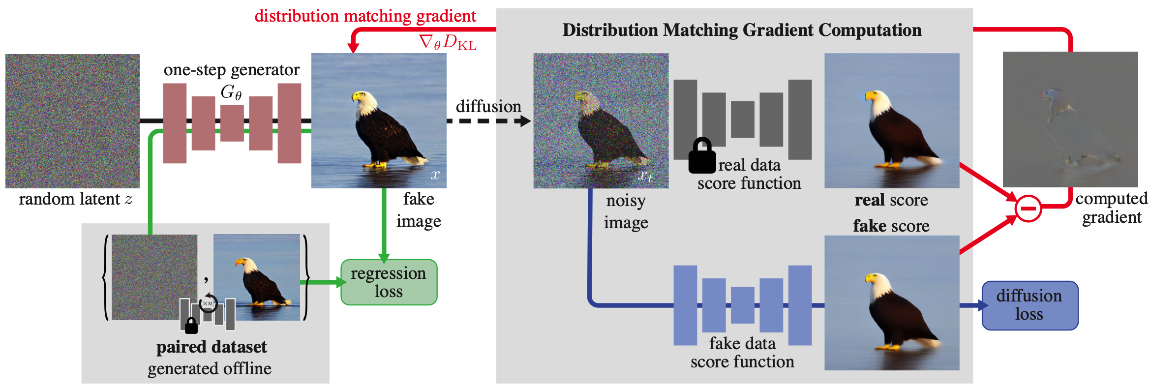
In essence, the motivation is to create one-step image generators that can achieve quality comparable to costly multi-step diffusion models while being orders of magnitude faster. DMD achieves this by introducing a distribution matching objective, bolstered by a regression loss, to efficiently distill knowledge from powerful diffusion models. The method aims to close the fidelity gap between distilled and base models while enabling 100x reduction in neural network evaluations and generating 512x512 images at 20 FPS.
Methodology
Notation
-
Given pretrained diffusion model $\mu_{\text{base}}$, that is able to generate data samples $x_0$ from noisy samples $x_T$ for $T$ steps.
-
$G_\theta$ is a one-step generator that has the architecture of the base diffusion denoiser but without time-conditioning. The authors initialize its parameters $\theta$ with the base model, i.e., $G_{\theta}(z) = \mu_{\text{base}}(z, T - 1), \quad \forall z$, before training. $T-1$ is the first step of generation.
-
The authors denote the outputs of the distilled model as fake, as opposed to the real images from the training distribution. It means that $G_{\theta}$ models $p_{\text{fake}}$ distribution while pretrained diffusion model $\mu_{\text{base}}$ models $p_{\text{real}}$ distribution.
Distribution Matching Loss
Ideally, a fast generator should produce samples that are indistinguishable from real images. To achieve this, the authors minimize the Kullback–Leibler (KL) divergence between the real and fake image distributions, $p_{\text{real}}$ and $p_{\text{fake}}$, respectively:
\[D_{KL}(p_{\text{fake}} \parallel p_{\text{real}}) = \mathbb{E}_{z \sim \mathcal{N}(0, I),\; x = G_{\theta}(z)} \left[ \log p_{\text{fake}}(x) - \log p_{\text{real}}(x) \right]\]Computing the probability densities to estimate this loss is generally intractable, but only the gradient with respect to $\theta$ is needed to train the generator by gradient descent:
\[\nabla_\theta D_{KL} = \mathbb{E}_{\substack{z \sim \mathcal{N}(0, I) \\ x = G_\theta(z)}} \left[ -\left(s_{\text{real}}(x) - s_{\text{fake}}(x)\right) \frac{dG}{d\theta} \right]\]$\text{where } s_{\text{real}}(x) = \nabla_x \log p_{\text{real}}(x), \quad s_{\text{fake}}(x) = \nabla_x \log p_{\text{fake}}(x)$. Since the expectation is taken only over the normal distribution, the expression under the expectation is differentiated.
Computing this gradient is still challenging for two reasons:
- first, the scores diverge for samples with low probability — in particular $p_{\text{real}}$ vanishes for fake samples,
- second, the intended tool for estimating score, namely the diffusion models, only provide scores of the diffused distribution.
So, the proposed strategy is to calculate a noisy score instead of a clean one. The scores $s_{\text{real}}(x_t, t)$ and $s_{\text{fake}}(x_t, t)$ are defined accordingly.
Diffused sample $x_t \sim q(x_t \mid x)$ is obtained by adding noise to generator output $x = G_\theta(z)$ at diffusion time step $t$: $q_t(x_t \mid x) \sim \mathcal{N}(\alpha_t x,\, \sigma_t^2 \mathbf{I})$.
The real score is modeled using pretrained diffusion model: $s_{\text{real}}(x_t, t) = - \frac{x_t - \alpha_t \mu_{\text{base}}(x_t, t)}{\sigma_t^2}$.
Fake score
The fake score function is derived in the same manner as the real score case: $s_{\text{fake}}(x_t, t) = - \frac{x_t - \alpha_t \mu^{\phi}_{\text{fake}}(x_t, t)}{\sigma_t^2}$.
However, as the distribution of the generated samples changes throughout training, the fake diffusion model $\mu^{\phi}_{\text{fake}}$ is dynamically adjusted to track these changes.
The authors initialize the fake diffusion model from the pretrained diffusion model $\mu_{\text{base}}$, updating parameters $\phi$ during training, by minimizing a standard denoising objective: \(\mathcal{L}^{\phi}_{\text{denoise}} = ||\mu^{\phi}_{\text{fake}}(x_t, t) - x_0||_2^2\)
where $\mathcal{L}^{\phi}_{\text{denoise}}$ is weighted according to the diffusion timestep $t$, using the same weighting strategy employed during the training of the base diffusion model.
\[\nabla_{\theta} D_{KL} \simeq \mathbb{E}_{z, t, x, x_t} \left[ w_t \alpha_t \left( s_{\text{fake}}(x_t, t) - s_{\text{real}}(x_t, t) \right) \frac{dG}{d\theta} \right]\]Distribution matching gradient update
where $z \sim \mathcal{N}(0; \mathbf{I})$, $x = G_{\theta}(z)$, $t \sim \mathcal{U}(T_{\min}, T_{\max})$, and $x_t \sim q_t(x_t \mid x)$.
Here, $w_t$ is a time-dependent scalar weight added to improve the training dynamics. The weighting factor is designed to normalize the gradient’s magnitude across different noise levels. Specifically, the mean absolute error is computed across spatial and channel dimensions between the denoised image and the input, setting:
\[w_t = \frac{\sigma_t^2}{\alpha_t} \cdot \frac{CS}{\left\| \mu_{\text{base}}(x_t, t) - x \right\|_1}\]where $S$ is the number of spatial locations and $C$ is the number of channels.
The authors set $T_{\min} = 0.02T$ and $T_{\max} = 0.98T$, following DreamFusion.
Torch computation of DMD loss
In order to get given gradient we could use the follwoing loss:
$L = \bigg( x - \big[x - (s_{\text{fake}}(x_t, t) - s_{\text{real}}(x_t, t))\big]\text{.detach()} \bigg)^2$
Then the gradient of $L$ will be exactly that we need:
$\nabla_{\theta} L = 2 \cdot (s_{\text{fake}}(x_t, t) - s_{\text{real}}(x_t, t)) \cdot \nabla_{\theta} x, \text{ where } x = G_{\theta}(z)$
Regression loss
The distribution matching objective is well-defined for $t \gg 0$, i.e., when the generated samples are corrupted with a large amount of noise. However, for a small amount of noise, $s_{\text{real}}(x_t, t)$ often becomes unreliable, as $p_{\text{real}}(x_t, t)$ goes to zero. Furthermore the optimization is susceptible to mode collapse, where the fake distribution assigns higher overall density to a subset of the modes. To avoid this, an additional regression loss is used to ensure all modes are preserved.
\[\mathcal{L}_{\text{reg}} = \mathbb{E}_{(z,y) \sim \mathcal{D}} \, \ell(G_{\theta}(z), y)\]This loss measures the pointwise distance between the generator and base diffusion model outputs, given the \textit{same} input noise. Concretely, the authors build a paired dataset $\mathcal{D} = {z, y}$ of random Gaussian noise images $z$ and the corresponding outputs $y$, obtained by sampling the pretrained diffusion model $\mu_{\text{base}}$ using a deterministic ODE solver. Learned Perceptual Image Patch Similarity (LPIPS) is used as the distance function.
Final objective
Network $\mu_{\text{fake}}^{\phi}$ is trained with \(\mathcal{L}^{\phi}_{\text{denoise}}\), which is used to help calculate $\nabla_{\theta} D_{KL}$. For training $G_\theta$, the final objective is: \(D_{KL} + \lambda_{\text{reg}} \mathcal{L}_{\text{reg}}, \quad \text{with} \quad \lambda_{\text{reg}} = 0.25\) unless otherwise specified.