Scalable emulation of protein equilibrium ensembles with generative deep learning
Motivation
Protein science can be characterized by three pillars of understanding: sequence, structure, and function.
- Sequence refers to the linear order of amino acids in the protein chain.
- Structure means the three-dimensional conformation (how the chain folds and organizes in space).
- Function describes what the protein does biologically (e.g., catalyzing a reaction, binding a ligand, transmitting a signal).
Function, being emerged from sequence and structure, is considered separately because:
- Two proteins can have similar folds (structural homology) but do very different things.
- Conversely, very different folds can evolve to perform similar functions (convergent evolution).
- Even subtle dynamic features, like conformational changes, can determine what a protein does.
- Function depends not only on static structure but on interactions with other molecules, post-translational modifications, cellular localization, and dynamics.
- For example: hemoglobin and myoglobin are structurally related but differ dramatically in oxygen transport vs. storage.
Functional descriptions such as “actin builds up muscle fibers” are human-made attributions that arise from objectively measurable mechanistic properties:
- What are the conformational states (i.e., sets of different structures) a protein can be in?
- Which other molecules can a protein bind to in these different conformations?
- What is the probability of these conformational and binding states at a given set of experimental conditions?
Methodology
The entire pipeline consists of the following steps:
- The authors train a conditional Riemannian diffusion model on the coordinates of $C_{\alpha}$ atoms.
- As a condition, the diffusion model receives a sequence embedding, which is derived from AlphaFold.
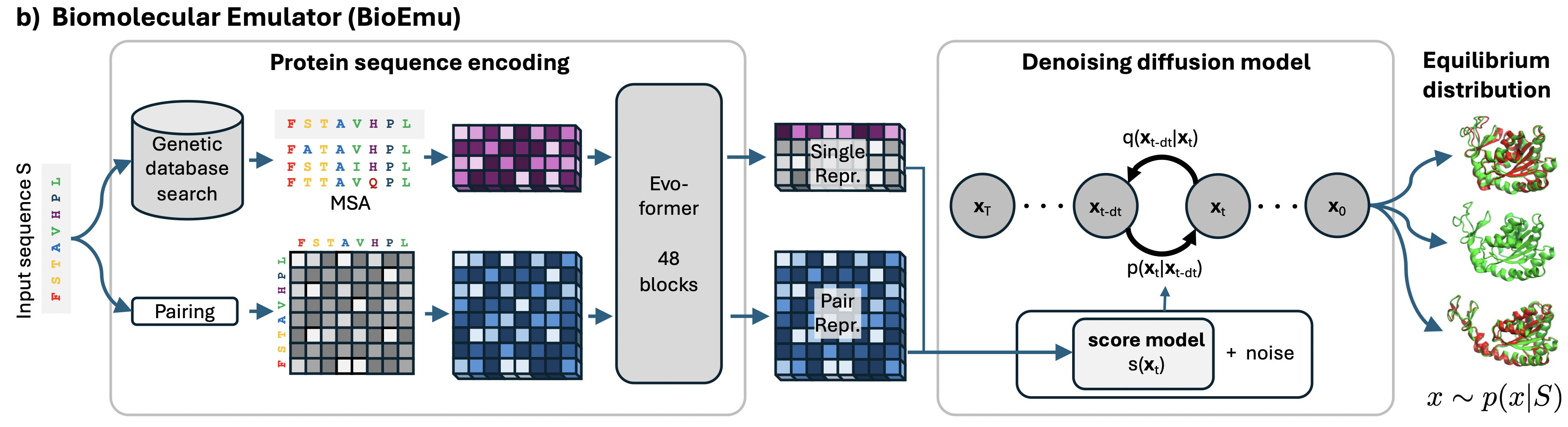
Diffusion Model
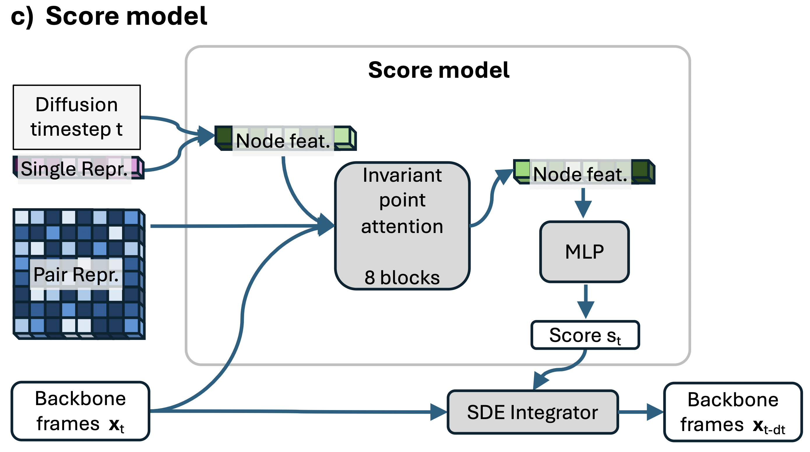
Protein Sequence Encoder
The protein sequence $S$ is encoded through the protein sequence encoder to compute single and pair representations using a simplified version of AlphaFold2.
Training Methodology
- The authors first train on a synthetic dataset derived from AFDB, with high sequence diversity and varied conformations for each sequence. The pretrained model can predict diverse conformations for the same protein sequence, but does not quantitatively match the probabilities of different states.
- That’s why they fine-tune on 95% MD simulation data and folding free energy measurements, mixed with 5% AFDB structures.
Data Splitting
Having defined a list of test proteins, authors removed from training and validation data any protein whose sequence was similar to any test protein’s sequence. Specifically, they used the mmseqs2 software (version 15.6f452) and removed proteins if they have 40% or higher sequence similarity with any test protein of at least 20 residues in size, using the highest sensitivity parameter supported by the software.
Pre-training on AFDB
Preprocessing steps:
- Using mmseqs Cluster all sequences of AFDB at $80%$ sequence identity and $70%$ coverage, resulting in a set containing more than 93 million clusters.
- Get a set of sequence clusters with 80% sequence similarity within each cluster and at most 30% sequence similarity between the centroids of different clusters. To do this they
- Cluster all the centroids of these clusters at $30%$ sequence identity.
- Leave only one centroid and its corresponding cluster in the entire centroid-cluster (typically the largest cluster). Intuitively: If several 80% clusters are similar, one representative is sufficient: the others carry almost the same information and can be discarded.
- Discard sequence clusters with fewer than 10 members, leaving roughly 1.4 million sequence cluster.
- Then they perform structure-based clustering.
- They cluster each sequence cluster using foldseek with a sequence identity threshold of $70%$ at $90%$ coverage.
- Then they discarded everything except the representative member of each structure cluster, leaving a few structure representatives for each sequence cluster.
- Then they discarded all sequence cluster with single structure representative and those where all the structure representatives were disordered (defined as being composed of more than 50% coil in their secondary structure).
- To exclude similar structure with missing regions which were flagged incorrectly they discarded structure representative if it has TM-score greater than $0.9$ to another structure representative.
- They additionally remove sequence clusters lacking at least one structure representative with pLDDT greater than 80, and with a pLDDT standard deviation lower than 15 across residues.
After running this pipeline, they had∼50k sequence clusters with structural diversity.
To draw training examples from this dataset, we randomly select a sequence cluster, and then a structure from within that cluster.
While the structure is randomly selected, we always use the sequence associated with the highest pLDDT structure in the cluster as input to the model. This effectively creates a mapping from a sequence to multiple structures.
Finetuning
The authors collect a bunch of datasets from molecular dynamic and finetune their model on this data. They sampled from each finetuning dataset qwith predefined probability. By finetuning was done in the same way as pretraining.
So on this stage they just git a model that could sample diverse structures for single sequence but without need probability.
Metrics
Coverage
Intuition:
Imagine you have a set of “target points”—these are the experimental 3-D conformations of the same protein. You generate a thousand (or more) predicted structures—these are the “darts.” The coverage metric answers the question: “How many of the reference targets have at least a few darts landing sufficiently close?”
How It Is Calculated:
- Select a Proximity Metric: Typically, this is RMSD, but it could also be TM-score, contact map, etc.
- Evaluate Each Reference Conformation: For each reference conformation, examine all predicted samples to find if any are within the chosen distance threshold.
- Avoid Random Matches: To ensure a match isn’t random, at least 0.1% of samples (i.e., ≥ 1 out of ~1000) must be within the threshold. If there are 10,000 samples, at least 10 “hits” are required.
- Determine Coverage: If the condition is met, the conformation is considered covered. Coverage is calculated as the number of covered conformations divided by the total number of reference conformations.
This process yields a coverage-versus-threshold curve: the stricter the threshold (lower RMSD), the harder it is to “cover” all targets, resulting in lower coverage.
Evaluation
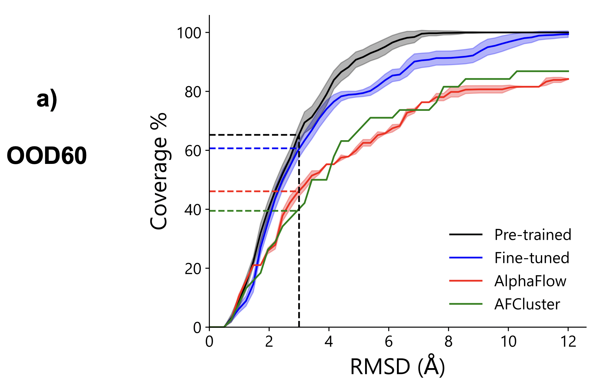
The authors assess whether BioEmu can qualitatively sample biologically relevant conformations and compare it to AFCluster and AlphaFlow baselines. They created a challenging test set, OOD60, consisting of 19 proteins with strict sequence similarity limits (60% and 40%) to AlphaFold2 and their training data. OOD60 includes difficult cases such as large conformational changes due to binding. Although predicting all these changes with a single-domain model is uncertain, BioEmu shows much better performance than the baselines in generalization benchmarks.