De novo design of protein structure and function with RFdiffusion
Receipt of RFDiffusion
- Pre-train the model on the task of generating protein structures from sequences.
- Train two flow diffusion model: Riemannian diffusion for residue rotation matrices and Gaussian diffusion for residue translations.
- Use self-conditioning for better generation.
RoseTTAFold Modifications
Architecture
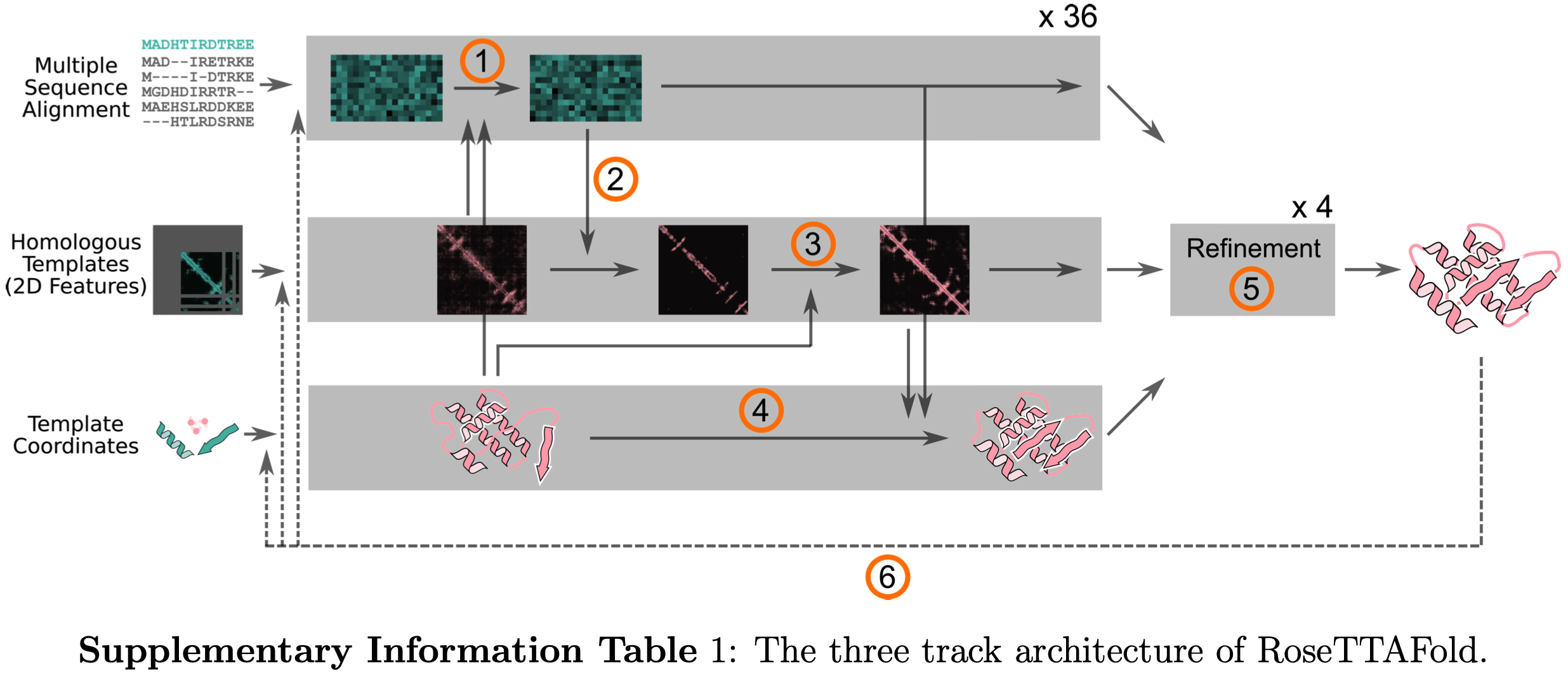
RFDiffusion has repurposed RoseTTAFold as the neural network in a diffusion model of protein backbones.
RFDiffusion Methodology
RF adopts a rigid-frame representation of the residues that comprise protein backbones. The structure of an $L$ residue backbone is described as a collection of residue frames $ x = [x_1, \dots, x_L]$, where each $x_l = (r_l, z_l)$ describes the translation $z_l \in \mathbb{R}^3$ and rigid rotation $r_l$ of the $l^{\text{th}}$ residue.
Diffusion Process
The reverse process transitions are modeled as conditionally independent across rotational and translational components.
The entire generation process can be divided into two independent components: a Gaussian transition for the translational component and an update for the rotational component. Since rotation matrices belong to the group SO(3), the generation is carried out as follows: at each step, we project r_t onto the tangent plane, take a step in the direction of the score, and then map the resulting point back to the SO(3) space.
Residue translations
As translation is just a point in the space it could be modelled using standard gaussian diffusion.
Residue rotations
$r_l$ is a rotation matrix. 3D rotation group, SO(3), is the group of all rotations in \(\mathbb{R}\) under the operation of composition.
Our aim in this section is to define the process of rotation corruption in order to build diffusion model.
For the forward and reverse transitions on rotations, we adapt a generalization developed by De Bortoli et al. of diffusion models to Riemannian manifolds.
Forward process defined by Brownian motion on SO(3)
Define an inner-product on the associated tangent spaces $\tau_r$. For any $r \in$ SO(3) and $A, B \in \tau_r$:
\[\langle A, B \rangle\_{SO(3)} = \mathrm{Trace}(A^\top B)/2\]The marginal distribution of a rotation matrix $r^(t)$ evolving according to Brownian motion for time $t$ from an initial rotation $r^(0)$ is given by the isotropic gaussian distribution $\mathcal{IG}_{\text{SO(3)}}$:
\[r^{(t)} \sim \mathcal{IG}_{SO(3)}\left( \mu = r^{(0)}, \, \sigma^2 = t \right)\] \[\mathcal{IG}_{SO(3)}(r^{(t)}; \mu, \sigma^2) = f\big(\omega(\mu^\top r^{(t)}); \sigma^2\big),\] \[f(\omega; \sigma^2) = \sum_{l=0}^{\infty} (2l + 1) e^{-l(l+1)\sigma^2 / 2} \frac{\sin\big((l + \tfrac{1}{2}) \omega\big)}{\sin(\omega / 2)}\]where $\mu$ is a $3 \times 3$ mean rotation matrix and $\omega(r)$ denotes the angle of rotation in radians associated with a rotation $r$. The angle may be computed as \(\omega(r) = \arccos\left( \frac{\mathrm{trace}(R) - 1}{2} \right)\).
Backward transition kernel
To approximate the reverse transitions for the rotations we take inspiration from De Bortoli et al. [Theorem 1] and approximate the discretized reversal by a geodesic random walk.
In particular, reverse step updates for rotations are computed by taking a noisy step in the tangent space of SO(3) in the direction of the gradient of the log density of a noised structure $x(t)$ with respect to each rotation, and projecting back to the SO(3) manifold using the exponential map.
The tangent space of SO(3) is \(\mathfrak{so}(3) = \bigl\{ A \in \text{Mat}\_{3 \times 3}(\mathbb{R}) \mid A^{\top} = -A \bigl\}\) at point $I_3$ (identity rotation).
\(\mathfrak{so}(3)\) has orthonormal basis:
\[f_1 = \begin{pmatrix} 0 & 0 & 0 \\ 0 & 0 & -1 \\ 0 & 1 & 0 \end{pmatrix}, \quad f_2 = \begin{pmatrix} 0 & 0 & 1 \\ 0 & 0 & 0 \\ -1 & 0 & 0 \end{pmatrix}, \quad f_3 = \begin{pmatrix} 0 & -1 & 0 \\ 1 & 0 & 0 \\ 0 & 0 & 0 \end{pmatrix},\]For every other point $ r \in $ SO(3), $\tau_r$ (tangent space at point $r$) has orthonormal basis \(\bigl\{ rf_1, rf_2, rf_3 \bigl\}\).
Each step of the geodesic random walk is computed as:
\[\begin{equation} r^{(t-1)} = \exp_{r^{(t)}} \bigl\{ (\sigma_t^2 - \sigma_{t-1}^2)\nabla_{r^{(t)}} \log q(x^{(t)}) + \sqrt{\sigma_t^2 - \sigma_{t-1}^2} \sum_{d=1}^{3} \epsilon_d r^{(t)} f_d \bigl\}, \tag{7} \end{equation}\]where
-
$\nabla_{r^{(t)}} \log q(x^{(t)})$ in \(\mathcal{T}_{r^{(t)}}\) denotes the Stein score of the forward process at time $t$,
-
$\exp_{r^{(t)}}$ denotes the exponential map from \(\mathcal{T}_{r^{(t)}}\) to $SO(3)$, (reverse mapping from tangent space to $SO(3)$). The exponential map $\exp_{r^{(t)}}$ may be computed as $\exp_{r^{(t)}}{v} = r^{(t)} \exp_{I_3}{r^{(t)\top}v}$, where $\exp_{I_3}$ is the matrix exponential.
-
$\epsilon_1, \epsilon_2, \epsilon_3 \overset{iid}{\sim} \mathcal{N}(0, 1)$.
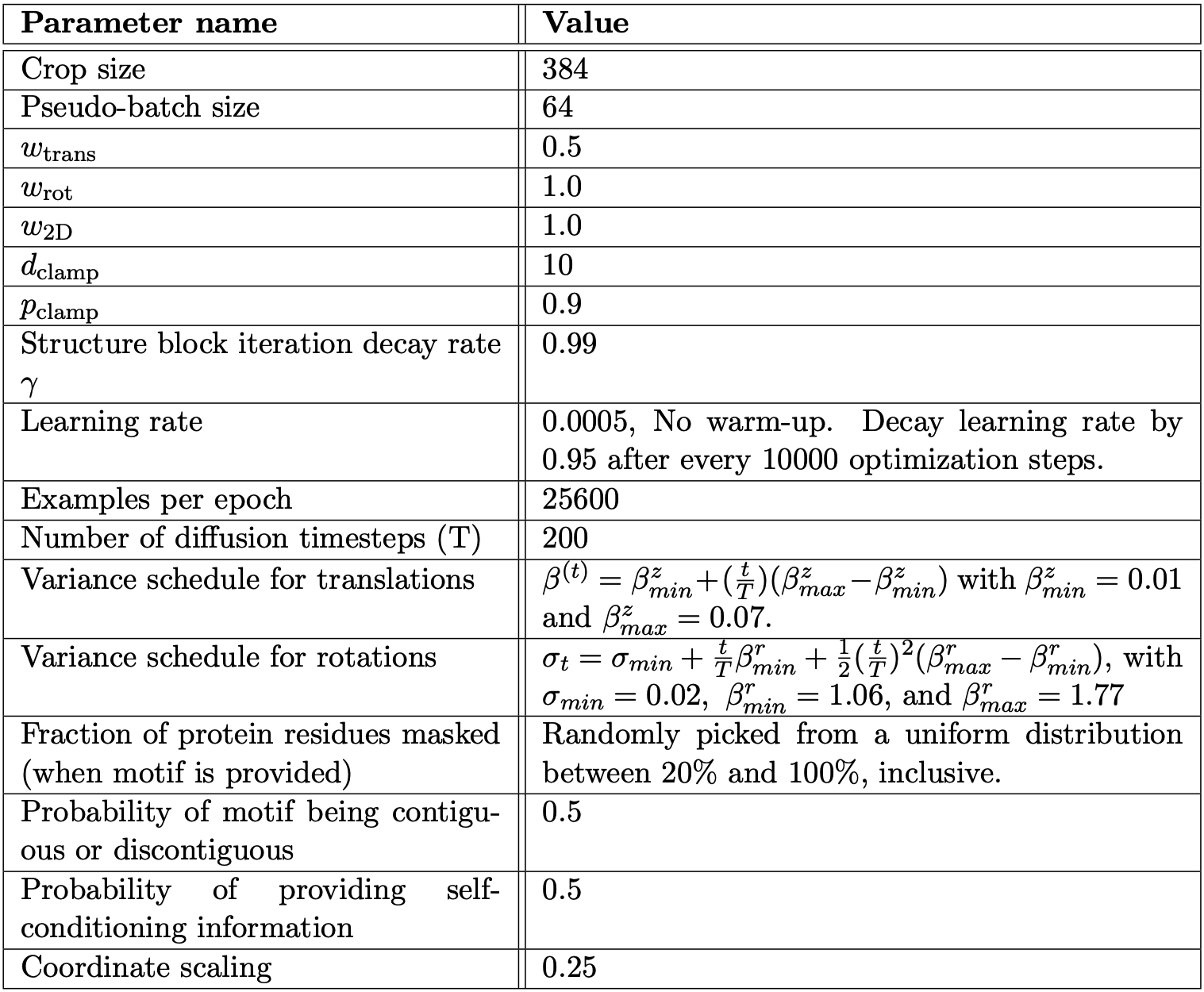
The variance schedule for the rotations is chosen by setting \(\sigma_t = \sigma_{\min} + \frac{t}{T} \beta_{\min} + \frac{1}{2} \left( \frac{t}{T} \right)^2 (\beta_{\max}^r - \beta_{\min}^r)\) with $\sigma_{\min} = 0.02$, $\beta_{\min}^r = 1.06$, and $\beta_{\max}^r = 1.77$.
Approximating the score with a denoising prediction
Instead of using score matching objective authors rely on score approximation that directly leverages RoseTTAFold’s ability to predict denoised structures. For a given $t$ and $r^{(t)}$:
\[\begin{align*} \nabla_{r^{(t)}} \log q(x^{(t)}) &= \mathbb{E}_q \nabla_{r^{(t)}} \log \frac{q(x^{(t)} \mid x^{(0)}) \cdot q(x^{(0)})}{q(x^{(0)} \mid x^{(t)})} \\ &= \mathbb{E}_q \left[ \nabla_{r^{(t)}} \log q(x^{(t)} \mid x^{(0)}) - \nabla_{r^{(t)}} \log q(x^{(0)} \mid x^{(t)}) \right] \\ &= \mathbb{E}_q \left[ \nabla_{r^{(t)}} \log q(x^{(t)} \mid x^{(0)}) \right] - \mathbb{E} \left[ \nabla_{r^{(t)}} q(x^{(0)} \mid x^{(t)}) \right] \\ &= \mathbb{E}_q \left[ \nabla_{r^{(t)}} \log q(x^{(t)} \mid x^{(0)}) \right], \text{as component are independent} \\ &= \mathbb{E}_q \left[ \nabla_{r^{(t)}} \log q(r^{(t)} \mid r^{(0)}) \right] \\ &\approx \nabla_{r^{(t)}} \log q(r^{(t)} \mid r^{(0)} = \hat{r}^{(0)}) \\ &= \nabla_{r^{(t)}} \log \mathcal{IG}_{SO(3)}(r^{(t)}; \hat{r}^{(0)}, \sigma_t^2), \end{align*}\]where denoised rotation is predicted by RFDiffusion.
Self-conditioning in reverse process sampling
With self-conditioning one saves the denoising predictions at each step and provides them as an input to the denoising model at the next iteration, instead predicting $\hat{x}^{(0)}(x^{(t)}, \hat{x}^{(0)}_{\text{prev}})$.
Training Details
RFDiffusion is initialized with pretrained RoseTTAFold weights.
Losses
\[\mathcal{L}_{\text{Diffusion}} = \mathcal{L}_{\text{Frame}} + w_{\text{2D}} \mathcal{L}_{\text{2D}},\]1. Primary loss
\[\text{MSE}_{\text{Frame}} = \mathbb{E}_{t, x^{(0)}} \left[ d_{\text{frame}}\left(x^{(0)}, \hat{x}^{(0)}(x^{(t)})\right)^2 \right],\] \[d_{\text{frame}}(x^{(0)}, \hat{x}^{(0)}) = \sqrt{ \frac{1}{L} \sum_{l=1}^{L} \left\| z_l^{(0)} - \hat{z}_l^{(0)} \right\|_2^2 + \left\| I_3 - \hat{r}_l^{(0)\top} r_l^{(0)} \right\|_F^2 },\]2. Modified loss
\(\mathcal{L}_{\text{Frame}}\) is a modified variant of squared distance loss.
It relies on a weighted sum of the translation and rotation components that includes clamping on translation distance:
\[d_{\text{Frame}}(x^{(0)}, \hat{x}^{(0)}) = \sqrt{ \frac{1}{L} \sum_{l=1}^{L} \left( w_{\text{trans}} \min\left( \left\| z_l^{(0)} - \hat{z}_l^{(0)} \right\|_2, d_{\text{clamp}} \right)^2 + w_{\text{rot}} \left\| I_3 - \hat{r}_l^{(0)\top} r_l^{(0)} \right\|_F^2 \right) }\]The translation distance is only clamped 90% of the time.
\(\mathcal{L}_{\text{Frame}}\) includes contributions from $d_{\text{Frame}}(x^{(0)}, \hat{x}^{(0)})$ computed at each intermediate model’s block with an exponential weighting, $\gamma$, that places greater importance on later outputs:
\[\mathcal{L}_{\text{Frame}} = \frac{1}{\sum_{i=0}^{I-1} \gamma^i} \sum_{i=1}^{I} \gamma^{I-i} d_{\text{Frame}}(x^{(0)}, \hat{x}^{(0),i})^2\]where $\hat{x}^{(0),i}$ is the $i^{\text{th}}$ structure block output.
For the second term in the loss, \(\mathcal{L}_{2}\), the model outputs multimodal distributions of expected distances, dihedral angles, and planar angles between all pairs of contacting residues. $D_{:,l,l’},\ \Omega_{:,l,l’},\ \Phi_{:,l,l’},\ \Theta_{:,l,l’}$ together describe the orientation of residue $l$ relative to residue $l’$. The following loss consists of the cross entropy between the one-hot histogram of the known inter-residue distances and orientations and the corresponding distributions predicted by the model.
\[\begin{align*} \mathcal{L}_{\text{2D}}(\text{logits}_d, \text{logits}_\omega, \text{logits}_\theta, \text{logits}_\phi, z_0) = & \text{CrossEntropy}(\text{logits}_{\text{dist}}, D) + \\ & \text{CrossEntropy}(\text{logits}_\omega, \Omega) + \\ & \text{CrossEntropy}(\text{logits}_\theta, \Theta) + \\ & \text{CrossEntropy}(\text{logits}_\phi, \Phi) \\ \end{align*}\]Hyperparameters