Highly accurate protein structure prediction with AlphaFold
AlphaFold Pipeline
The whole pipeline is aimed to generate protein backbone for protein sequence. So the input to the pipeline is a sequence of amino acids.
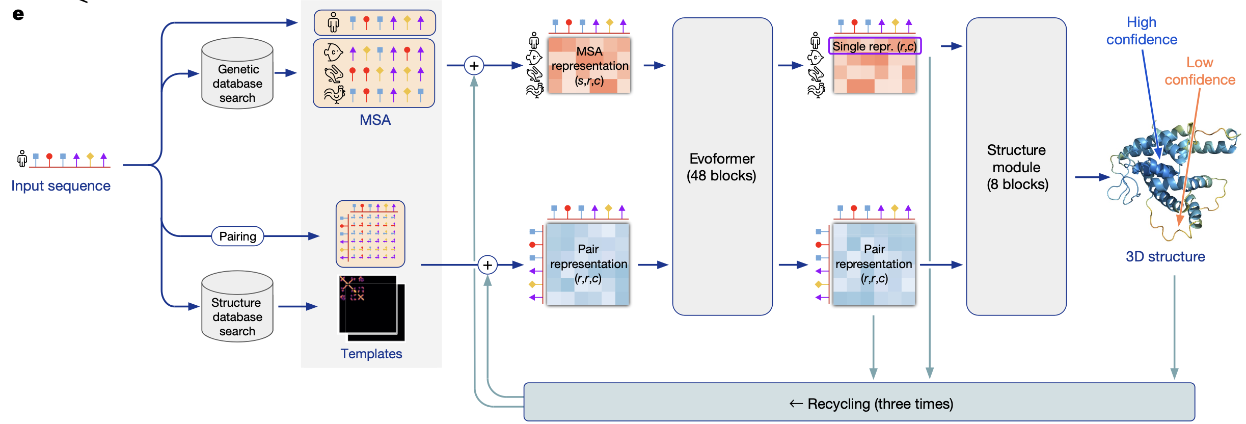
Genetic database search → retrieving evolutionary relatives
Fast profile/HMM tools such as JackHMMER, HHblits or MMseqs2 scan tens of millions of sequences (UniRef 90, UniProt, BFD, MGnify, Uniclust 30) for anything that is measurably homologous to your protein.
What is measurably homologous?
Homologous = from a common ancestor. Two protein (or DNA) sequences are called homologous when they ultimately descended from the same ancestral gene. That fact is binary—either they are or they aren’t—but we can only infer it from sequence data.
Practical rules of thumb
- Percent identity. Over a full-length alignment, ≥ 30 % identity is almost always enough to call two proteins homologous; below ~20 % you need profile or HMM methods to pick up the signal. pmc.ncbi.nlm.nih.gov
- Profile methods extend the range. T ools such as HHblits compare profiles (Hidden Markov Models) instead of raw sequences, letting you detect “remote” homology even when pairwise identity drops into the teens.
Why does it matter?
The more distant—but still related—sequences you can find, the richer the evolutionary signal you get. This operation returns a list of homologous sequences, a large pool of sequences that “know” something (through evolution) about how your protein folds.
Multiple Sequence Alignment (MSA) → organising those relatives into columns
1. Lines the hits up residue-by-residue so that amino acids performing the same functional/structural role sit in the same column.
Think of a protein sequence as a long sentence where each amino-acid “word” has a job. When we build a multiple-sequence alignment (MSA), we try to line sentences up so that the words that play the same part of the sentence—subject, verb, object—appear in vertical columns. In the protein world, that means:
| Functional / Structural "Job" | What the Residue Is Doing | Example |
|---|---|---|
| Catalysis (chemical work) | Directly takes part in the reaction—often found in enzyme active sites. | The Serine in the catalytic triad of serine proteases. |
| Ligand / metal binding | Holds on to a co-factor, metal ion, small molecule, DNA, another protein, etc. | The two Histidines and one Glutamate that chelate zinc in carbonic anhydrase. |
| Structural scaffolding | Packs into the hydrophobic core, forms a disulphide bridge, or acts as a hinge/turn that lets the protein fold properly. | A buried Leucine in a helix bundle; a Glycine in a β-turn. |
| Signal or recognition patch | Forms part of a surface motif recognised by other molecules. | The RGD motif (Arg-Gly-Asp) that integrins recognise. |
When the alignment is correct, every row in a given column traces back to the same position in the common ancestor of all those proteins, so the residues in that column:
- Sit at the same 3-D spot in the folded structure, and
- Usually have the same job (catalysis, binding, packing, flexibility, etc.).
That’s why you often see:
- Conserved columns: the exact amino acid hardly changes because the role is intolerant to mutation (e.g., catalytic Ser).
- Variable but chemically similar columns: the individual letters differ, but they share properties—say, all hydrophobic—because any residue that behaves the same is good enough for that structural slot.
So in the sentence you quoted, “amino acids performing the same functional/structural role” means residues that occupy equivalent positions in homologous proteins and therefore contribute in equivalent ways to what the protein does or how it folds. Lining them up in the same column lets AlphaFold (or any analysis) read the evolutionary record of which jobs are critical and which can flex.
Example
TODO
2. Encodes the MSA into a 3-D tensor called the "MSA representation" with axes (sequence, residue position, feature channels).
Each cell gets an embedding vector; AlphaFold treats the first row (your query) as a special “single representation” and keeps the rest as contextual rows.
This tensor is the main input to the Evoformer block.
Pairing → initialization of contact representation
Build an initial L × L feature matrix that simply tells the network how far apart residues are in sequence.
Think of it as a very lightweight spatial prior (positional information) before any structural reasoning happens. Without this, the model would have to discover contacts from scratch, making learning far harder.
Structure database search → templates
- AlphaFold runs a sequence‑profile search (HHsearch/HHblits) against a curated, non‑redundant slice of the Protein Data Bank (often called “PDB 70/100” because similar chains are clustered at 70 % or 100 % identity). So the search key is still the amino‑acid sequence, not 3‑D shape similarity. The hit list may include very remote homologues whose sequences share only 15–20 % identity with yours, because profile–profile matches can detect distant evolutionary relationships.
2. For the top ~20 alignments that pass an E‑value & coverage threshold, AlphaFold copies the template's backbone coordinates and encodes the inter‑residue distances/orientations into fixed‑size bins.
This geometric information is what eventually feeds into the pair representation and gives the network concrete spatial hints, especially in regions where the multiple‑sequence alignment (MSA) is thin.
E-value (expect value)
It measures a chance of meeting the sequence with aligment score bigger than given one in the whole database.
Formal definition
$E = Kmne^{-\lambda S}$ (the Karlin-Altschul equation), where S is the raw alignment score, m and n are the effective lengths of the query and database, and K, λ are statistical constants for the scoring matrix.
Lower is better. E = 1 × 10⁻³ means you’d expect one false-positive hit in a thousand equally good database searches.
Coverage threshold
$ \text{Coverage} = \frac{\text{aligned residues}}{\text{query length}}$. A spectacular E-value is useless if it aligns only a tiny fragment—that fragment may not be relevant to the overall fold you want to model.
Why both thresholds are used together
- E-value guards against false positives (bad statistics).
- Coverage guards against trivial positives (tiny true alignments that are uninformative for structure).
Only hits that pass both filters are promoted to “template” status; their atomic coordinates are then converted to the distance-and-orientation bins that seed the pair representation.
Why it matters
Many regions of a protein don’t have strong co‑evolutionary signal in the MSA. A template provides direct geometric hints there (backbone distances, side‑chain orientations). Templates help the network converge faster and are especially valuable for β‑sheet topologies that are hard to infer from sequence alone. Inside the model these coordinate‑based features are converted to a 2‑D array (distance & orientation bins) and added into the initial pair representation (the blue square in the diagram).
Evoformer
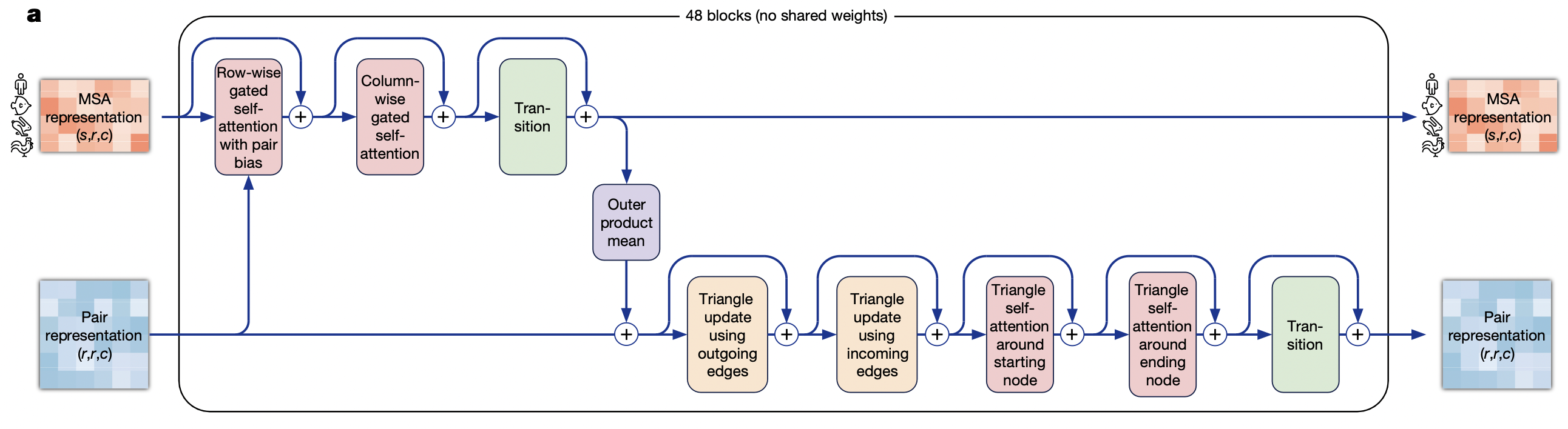
1. Row‑wise gated self‑attention with pair bias.
- What it does. For every single sequence (row) in the MSA, apply self‑attention along the residue axis.
- Why “pair bias”. The attention logits get an additive term derived from the current pair embedding for (i, j), so each sequence row is “aware” of the model’s latest guess about how residues i and j interact.
- Why “gated”. A learned sigmoid gate scales the output, letting the network suppress noisy signals when the alignment at that row is poor.
- Motivation. Propagate long‑range context within each homolog while conditioning on emerging structural hints.
Algorithm: Row‑wise Gated Self‑Attention with Pair Bias (single head $h$)
Inputs:
\[\begin{align*} \mathbf{M} &\in \mathbb{R}^{S \times L \times d_m} && \text{(current MSA embeddings)}\\ \mathbf{Z} &\in \mathbb{R}^{L \times L \times d_z} && \text{(current pair embeddings)}\\ W^Q,\,W^K,\,W^V &\in \mathbb{R}^{d_h \times d_m} && \text{(head‑specific projections)}\\ w^P &\in \mathbb{R}^{d_z} && \text{(projects pair features to scalar bias)}\\ W^O &\in \mathbb{R}^{d_m \times (H d_h)} && \text{(output projection)}\\ w^G &\in \mathbb{R}^{d_m},\; b^G \in \mathbb{R} && \text{(gate parameters)} \end{align*}\]- for $s = 1$ to $S$ do % row loop (one sequence)
- $\mathbf{Q} \leftarrow W^Q \, \mathbf{M}_{s,:,:}^{\!\top}$ % shape $d_h\times L$
- $\mathbf{K} \leftarrow W^K \, \mathbf{M}_{s,:,:}^{\!\top}$
- $\mathbf{V} \leftarrow W^V \, \mathbf{M}_{s,:,:}^{\!\top}$
- for $i = 1$ to $L$ do % token loop (residue $i$)
- for $j = 1$ to $L$ do
- $b_{ij} \leftarrow (w^P)^\top \mathbf{Z}_{ij}$ % pair‑bias
- $e_{ij} \leftarrow \dfrac{\mathbf{Q}_{:,i}^{\!\top} \mathbf{K}_{:,j}}{\sqrt{d_h}} + b_{ij}$ % logits
- end for
- $\boldsymbol{\alpha}_{i} \leftarrow \operatorname{softmax}(\mathbf{e}_{i,:})$ % over $j$
- $\mathbf{o}_i \leftarrow \displaystyle\sum_{j=1}^{L} \alpha_{ij}\, \mathbf{V}_{:,j}$ % weighted sum
- $g_i \leftarrow \sigma\bigl((w^G)^\top\mathbf{M}_{s,i,:} + b^{G}\bigr)$ % gate scalar
- $\widetilde{\mathbf{o}}_i \leftarrow g_i\,\mathbf{o}_i$ % apply gate
- $\mathbf{M}_{s,i,:} \leftarrow \mathbf{M}_{s,i,:} + W^{O}\widetilde{\mathbf{o}}_i$ % residual
- for $j = 1$ to $L$ do
- end for
- end for
2. Column‑wise gated self‑attention.
- What it does. Now fix a residue position r and attend down the column across the s sequences.
- Motivation. Let each residue in the target sequence look at how that same position varies (or co‑varies) across evolution, capturing conservation and compensatory mutations.
- Complexity trick. Row‑ and column‑wise attention factorise a huge 2‑D attention ( s r × s r ) into two linear passes, cutting time and memory by ~O(s r)
3. Transition
- A two‑layer feed‑forward network (ReLU / GLU) applied to every (s, r) token independently — the same role a “Transformer FFN” plays after its attention layer.
- Purpose: mix features non‑linearly and give the model extra capacity.
4. Outer product mean
- How. For each residue pair $(i, j)$, take the embedding vectors $v_i, v_j$ from every sequence, form the outer product $v_i \bigotimes v_j$ (a matrix), then average over the $s$ sequences.
- What it produces. A rich co‑evolution feature saying “when residue $i$ mutates like this, residue $j$ mutates like that.”
- Where it goes. Added into the pair tensor, giving it evolutionary coupling signal.
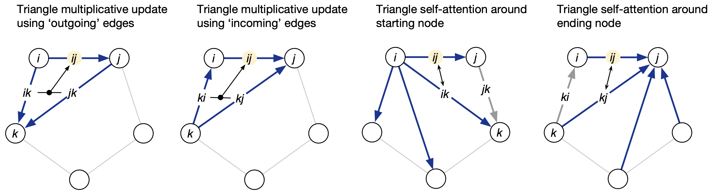
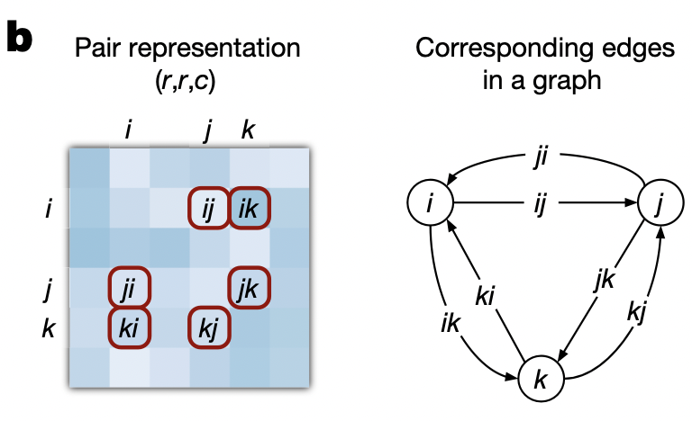
5. Triangle update using outgoing edges
- View the pair tensor as a fully‑connected directed graph of residues; each edge $(i, j)$ stores an embedding $z_{i, j}$.
- Update edge $(i, j)$ by multiplying / gating information that flows along the two edges $(i, k)$ and $(k, j)$ for every third residue $k$.
- Motivation: Impose triangle‑inequality‑like constraints and capture three‑body interactions essential for 3‑D geometry.
Algorithm
Let $\mathbf{Z} \in \mathbb{R}^{L \times L \times c}$ be the current pair tensor and let $i, j, k \in {1, \dots, L}$ index residues.
1. Project the two “arms” of each triangle
\[\begin{align*} & \mathbf{a}_{ik} &= W^{(a)} \mathbf{z}_{ik} \in \mathbb{R}^{c_m}, && \text{($i \rightarrow k$ arm)} \\ & \mathbf{b}_{kj} &= W^{(b)} \mathbf{z}_{kj} \in \mathbb{R}^{c_m}, && \text{($k \rightarrow j$ arm)} \end{align*}\]- $W^{(a)}, W^{(b)} \in \mathbb{R}^{c_m \times c}$ are learned linear maps.
- The projection width $c_m$ is usually $c/2$ so the outer product that follows keeps the channel count $\approx c$.
2. Form the triangle message for edge $(i, j)$:
\[\begin{align*} \quad \mathbf{t}_{ij} = \sum_{k=1}^{L} \frac{\mathbf{a}_{ik} \odot \mathbf{b}_{kj}}{\sqrt{L}} \in \mathbb{R}^{c_m} \end{align*}\]- Element-wise product $\odot$ mixes the two arms.
- Division by $\sqrt{L}$ is a variance-stabilising scale (analogous to the $1/\sqrt{d}$ in self-attention).
3. Transform, gate and add as a residual
\[\begin{align*} & \mathbf{u}_{ij} = W^{(o)} \mathbf{t}_{ij} \in \mathbb{R}^{c} \\ & g_{ij} = \sigma\left( (\mathbf{w}^{(g)})^\top \mathbf{z}_{ij} + b^{(g)} \right) \in (0, 1) \\ & \mathbf{z}'_{ij} = \mathbf{z}_{ij} + g_{ij} \, \mathbf{u}_{ij} \\ \end{align*}\]- $W^{(o)} \in \mathbb{R}^{c \times c_m}$ projects back to the original channel size.
- $g_{ij}$ is a sigmoid gate computed from the pre-update edge; it lets the network down-weight noisy triangles.
- The final line is a residual connection identical in spirit to the one in a Transformer block.
4. Vectorised Form
If we reshape $\mathbf{Z}$ to a 3-D tensor and use matrix multiplication, the whole operation is:
\[\begin{align*} \mathbf{Z} \leftarrow \mathbf{Z} + \sigma\left( \langle \mathbf{Z}, \mathbf{w}^{(g)} \rangle + b^{(g)} \right) \odot W^{(o)} \left( \frac{\mathbf{A} \odot \mathbf{B}}{\sqrt{L}} \mathbf{1} \right) \end{align*}\]with $\mathbf{A} = W^{(a)} \mathbf{Z}, \quad \mathbf{B} = W^{(b)} \mathbf{Z}$ and the sum over $k$ is implemented by a batched tensor contraction.
Intuition
- The update $\textbf{looks along paths}$ $i \rightarrow k \rightarrow j$ (“out-going” edges from $i$).
- It injects $\textit{multiplicative}$ three-body information, helping the network encode triangle inequalities and side-chain packing constraints—something plain pairwise couplings cannot capture.
6. Triangle update – using incoming edges
Same operation but centred on the opposite vertex, so the model sees both orientations of every residue triplet.
7. Triangle self‑attention around starting node
- Treat all edges that emanate from residue i as the “tokens” of an attention layer; use edge $(i, j)$ as the query and the set { $(i, k)$ } as keys/values.
- Learns patterns like “edges from this residue fan out in a β‑sheet vs. coil”.
8. Triangle self‑attention around ending node
- Same again but for edges that end at residue j. Together, the two triangle‑attention layers let the model reason about local geometry from both directions.
9. Transition
- A second feed‑forward network, now on every $(i, j)$ edge, to consolidate the information distilled by the triangle operations before looping to the next Evoformer block.
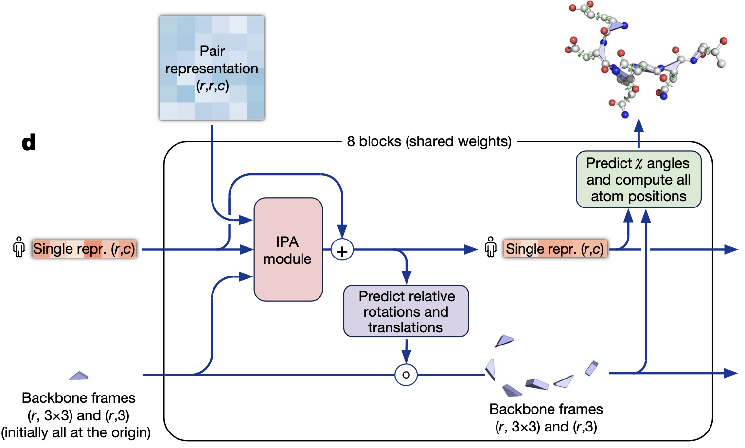
Structure Module
Input
| Tensor | Shape | What it encodes |
|---|---|---|
| Single representation S | (L, cs) | A per-residue feature vector distilled from the Evoformer. |
| Pair representation Z | (L, L, cz) | Rich geometry couplings (distances, orientations) between every residue pair. |
| Backbone frames {Ri, ti} | Ri ∈ SO(3), ti ∈ ℝ³ | One local 3-D coordinate frame per residue. Initialised as identity + zero, i.e. every residue sits at the origin pointing the same way. |
All three are recycled from the previous passes of AlphaFold; on the very first pass the frames are just those trivial identities.
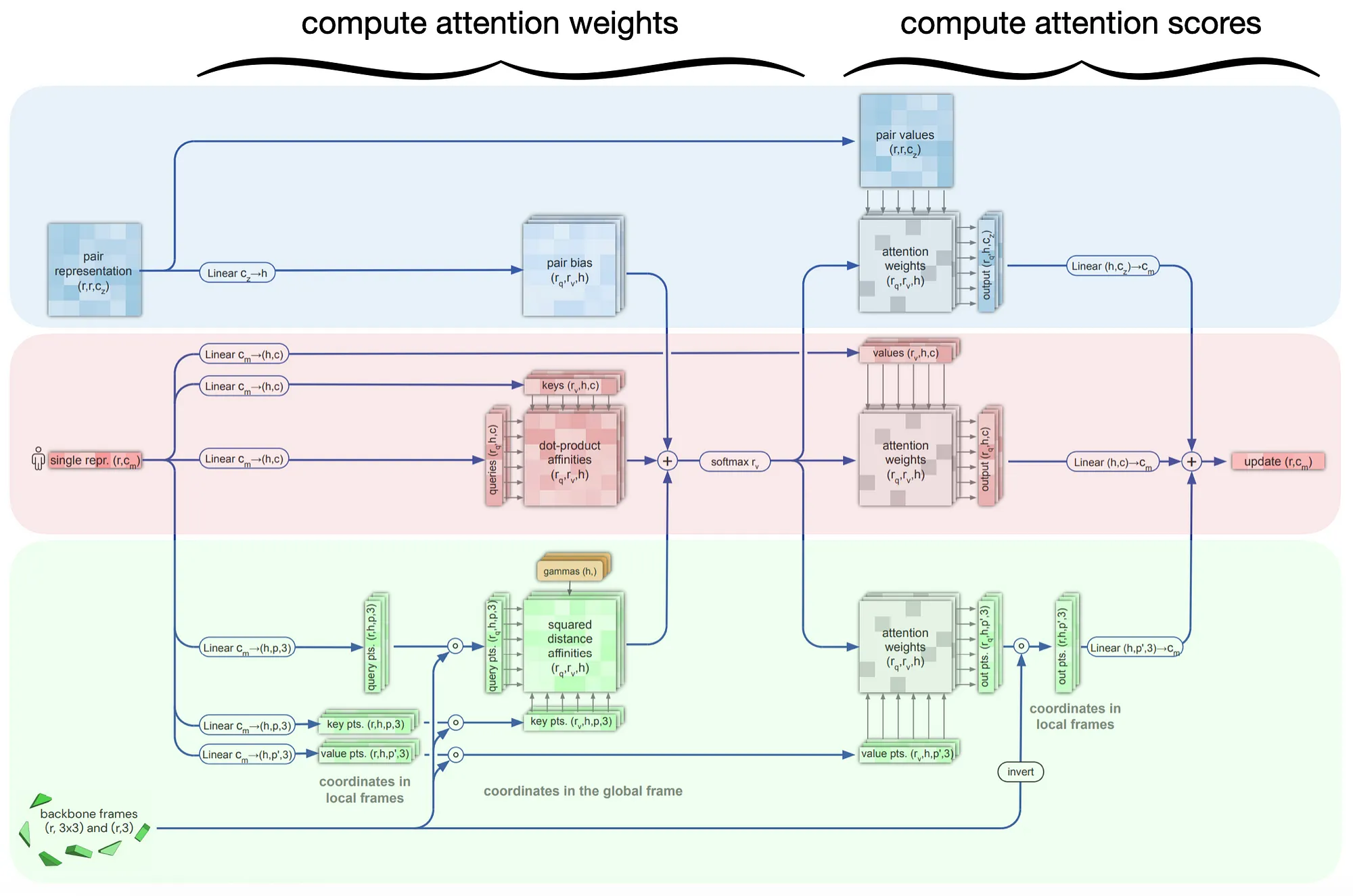
1. Invariant‑Point Attention (IPA)
IPA is the SE(3)‑equivariant replacement for the dot‑product attention you know from Transformers. The scalars (queries Q, keys K, values V) work almost exactly as usual, but every token (here: every residue i) is also equipped with a handful of small 3‑D point clouds that move rigidly with the residue’s current backbone frame.
2. Rigid‑body update head
A small MLP reads the new $S_i$ and predicts a delta rotation $\Delta R_i \in SO(3)$ (parameterised as a quaternion or axis–angle) and a delta translation $\Delta \mathbf{t}_i \in \mathbb{R}^3$.
\[\begin{align*} R_i \leftarrow \Delta R_i R_i, \qquad \mathbf{t}_i \leftarrow \mathbf{t}_i + \Delta \mathbf{t}_i \end{align*}\]Both deltas are passed through tanh-gated scales so that early iterations make only gentle moves; later passes can refine with larger steps.
3. Side‑chain / χ‑angle head
After the 8-th shared block, a final head predicts \textbf{torsion angles} $\chi_1, \chi_2, \ldots$ per residue.
The angles are applied to idealised residue templates stored inside the network to produce \textbf{all heavy-atom coordinates} (including side chains and hydrogens).
Why these ingredients?
| Component | Motivation |
|---|---|
| Backbone frames | A rigid frame per residue turns geometry prediction into learning a smooth field of rigid bodies—exactly what protein backbones are. |
| Invariant-Point Attention | Extends vanilla attention so that queries, keys, values, and pair bias are all SE(3)-equivariant; lets the network reason directly in 3-D without breaking equivariance. |
| Rigid-body deltas | Predicting changes (Δ) rather than absolute coordinates keeps gradients stable and avoids large jumps. |
| Shared weights over 8 recycles | Memory-efficient unrolled optimisation: the same parameters are reused, but the inputs keep evolving, so the network effectively performs eight refinement steps. |
| Side-chain torsion head | Once backbone placement converges, side-chain packing is adjusted coherently with the learned χ-angle statistics from the PDB. |
Training Procedure
- “Seed” model: Train AlphaFold only on experimental PDB structures for ≈ 300 k optimiser steps (just under half of the full run).
- One‑off inference sweep: Run that seed model on all UniRef90 clusters that have no PDB hit (≈ 2 M clusters). Keep the single representative sequence for each cluster. This step gives you 3‑D coordinates, per‑residue pLDDT and a predicted TM‑score for every sequence. Time cost: a few days on the same TPU pod that trains the network.
- Filtering / re‑weighting: No hard pre‑training filter. Instead, add the predictions to a TFRecord and store pLDDT as a training weight: $w_i = (\frac{pLDDT_i}{100})^2$. High‑confidence residues (pLDDT≈90) get weight ≈ 0.8; low‑confidence ones (pLDDT≈30) get weight ≈ 0.1 and therefore contribute almost nothing to the loss.
- Merge & continue training: Resume the same optimiser state. At every step sample 75 % PDB, 25 % self‑distilled crops. Continue for another ≈ 400 k steps. Because the optimiser is not re‑initialised, you can think of this as “fine‑tuning on a bigger, noisy set while still seeing clean PDB data every batch.”
On‑the‑fly feature generation
-
MSA search: Uses jackhmmer (UniRef90), HHblits (BFD, Uniclust30), and MGnify metagenomes. To avoid frozen data, 20 % of the time one of those databases is randomly dropped; another 20 % the MSA is subsampled or shuffled.
-
Template search: Runs HHsearch against a PDB70 library; at training time the top‑hit template is kept only with p = 0.75 and otherwise discarded so the model learns to work template‑free.
-
Random cropping: If a protein exceeds 384 residues, a contiguous window of crop_size ∼ Uniform(256,384) is chosen; MSAs and templates are cropped consistently.
-
Masking loss (BERT‑style): 15 % of MSA tokens are replaced by a mask character; the network must reconstruct them (auxiliary MSA‑loss).
Recycling
# --- 0. Feature construction -----------------------------------------
S0, Z0 = msa_and_template_features(query)     # shapes as above
frames0 = make_identity_frames(L)             # all residues at origin

# --- 1. Recycle loop ---------------------------------------------------
for t in range(N_RECYCLE):                    # 3 during training
    # Evoformer: updates tensor representations
    S_t, Z_t = Evoformer(S0, Z0)

    # Structure: predicts backbone + side chains
    frames_t, plddt_t, pae_t = Structure(S_t, Z_t)

    # Stop-grad on everything but keep the tensors
    S0 = stop_gradient(S_t)
    Z0 = stop_gradient(
            concat(Z_t, bins_from(frames_t), pae_t, plddt_t) )
Only the last pass’s outputs receive gradient signals (so GPU/TPU memory is roughly that of one forward path).
| Without recycling | With recycling |
|---|---|
| Evoformer must convert raw MSA + template signal directly into an atomic model. | First pass produces a rough fold; the next pass can treat that fold as an extra template and “zoom in” on clashes, mis-packed loops, β-sheet registry, etc. |
| pLDDT/PAE confidence heads see only one sample. | Confidence from pass t steers pass t + 1: the model learns to trust high-pLDDT regions and re-work low-pLDDT ones. |
| CASP-level accuracy would require a deeper or larger net. | Three passes of a 48-layer Evoformer + 8-block Structure module reach < 1Å GDT-TS error on many domains, with shared parameters. |
pLDDT Prediction
AlphaFold2 does not compute its confidence score after it has finished the 3-D model. Instead, it trains the network to predict its own error at the same time that it predicts the structure. The result is the predicted Local Distance Difference Test score (pLDDT)—a per-residue estimate (0–100) of how well the Cα atoms of that residue will match the unknown “true” structure.
After the structure module finishes its last recycling step it produces a single representation vector $s_i$ for every residue i. Those vectors feed a tiny multilayer perceptron (MLP): LayerNorm → Linear → ReLU Linear → ReLU (128 hidden channels) Linear → Softmax → 50 logits Each logit corresponds to an lDDT bin that is 2 units wide (centres = 1, 3, 5 … 99). The network therefore returns a probability distribution $p_i(b)$ over the 50 bins for every residue.
For each residue $\text{pLDDT}i = \sum{b=1}^{50} p_i(b) v_b,$ where $v_b$ is the bin centre (again 1, 3, 5 … 99).
-
Ground truth: For every PDB training chain with resolution 0.1–3.0 Å (the high-quality subset), the lDDT-Cα of the final AlphaFold output against the experimental structure is computed and discretised into the same 50 bins.
-
Loss: A simple per-residue cross-entropy between the predicted distribution $p_i$ and the one-hot target vector $y_i$. The confidence loss is added to the main FAPE / torsion / distogram losses with its own weight. The cross-entropy between the one-hot target and the logits does back-propagate through the MLP into the single residue embedding and all weights below it (Structure-Module and Evoformer). Thus the network is encouraged to encode “how right am I likely to be?” in that embedding.
Why it works so well
- The single representation still encodes all the information that controlled the structure prediction—template alignment quality, MSA depth, invariant point attention activations, etc.—so the tiny head can learn a rich error model without ever “seeing” the experimental target during inference.
Finetuning Phase
Last 50 k steps switch to full‑length crops (no random window), enable violation loss, and freeze the MSA‑masking term to zero weight. Fine‑tune re‑centres the model on physically plausible stereochemistry that the coarse cropping sometimes breaks.
Losses
| # | Loss term | What is actually computed | Motivation | When / how it is used |
|---|---|---|---|---|
| 1 | Frame-Aligned Point Error LFAPE | Align each residue’s local frame (predicted ↔ true), square-clamped distance between corresponding atoms, then average. | Primary geometry driver: forces correct local geometry while being invariant to global rigid moves; keeps gradients stable. | Full 7.5 M steps, highest weight (initial ≈ 1.0, then uncertainty-learned). |
| 2 | Distogram Ldist | 64-bin cross-entropy on Cβ–Cβ (Cα for Gly) distance distributions. | Guides pair representation; stabilises early training and enables self-distillation. | Entire training run; weight ≈ 0.3–0.5. |
| 3 | Backbone & side-chain torsion Lχ | L2 loss on sine/cosine of φ, ψ, and χ1–4 angles. | Enforces stereochemistry; distances alone cannot lock correct rotamers or Ramachandran regions. | Applied layer-wise + final; moderate weight ≈ 0.3. |
| 4 | Masked-MSA reconstruction Lmsa | BERT-style token cross-entropy on 15 % masked MSA positions. | Self-supervision on evolutionary data; regularises and enriches sequence embeddings. | Whole training; small weight ≈ 0.1. |
| 5 | Confidence (pLDDT & pTM) Lconf | Cross-entropy (pLDDT) & MSE (pTM) against on-the-fly self-targets. | Teaches the model to calibrate its own error without pulling atoms directly. | All steps; tiny weight ≈ 0.01 (∼1 % of FAPE). |
| 6 | Violation Lviol | Penalties for bond/angle outliers, clashes, Ramachandran violations. | Injects basic chemistry; catches illegal geometries not covered by FAPE. | Only last ~50 k fine-tune steps; weight ≈ 0.3. |
Ablation
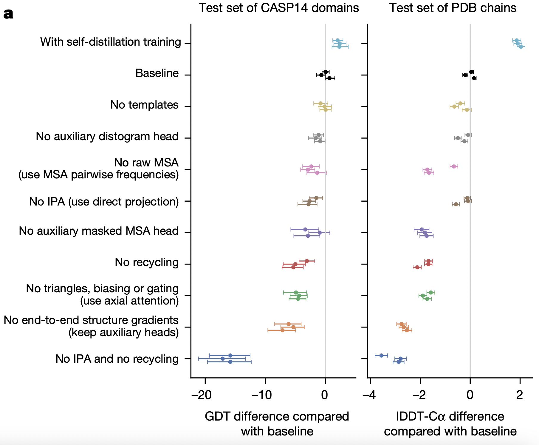
| Ablation experiment | Δ GDTTS (CASP14) | Δ lDDT‑Cα (PDB set) | Interpretation of the drop / gain |
|---|---|---|---|
| With self‑distillation data added | ≈ +1.5 | ≈ +0.2 | Extra pseudo‑labels expose far more sequence diversity, giving a modest but consistent boost. |
| No templates | ≈ ‑2 | ≈ ‑0.3 | Template signal helps only occasionally; AF2 is largely de novo, so the impact is small. |
| No auxiliary distogram head | ≈ ‑3 – 4 | ≈ ‑0.5 | Pair representation loses explicit distance supervision, hurting contact inference. |
| No raw MSA (use pair‑frequency matrix only) | ≈ ‑6 | ≈ ‑1.0 | Removing higher‑order co‑evolution erases much of the contact signal encoded in the MSA. |
| No Invariant Point Attention (direct projection) | ≈ ‑7 | ≈ ‑1.5 | Loses SE(3)‑equivariance; the structure module can’t reason about rotations/translations. |
| No auxiliary masked‑MSA head | ≈ ‑3.5 | ≈ ‑0.7 | Row‑wise representation is less regularised; long or sparse MSAs suffer most. |
| No recycling | ≈ ‑6 | ≈ ‑1.0 | A single pass cannot iron out clashes or register errors; iterative refinement is crucial. |
| No triangle updates, biasing or gating (use axial attention) | ≈ ‑7 | ≈ ‑1.3 | Weakens long‑range geometric reasoning that holds β‑sheets and domain interfaces together. |
| No end‑to‑end structure gradients (keep only auxiliary heads) | ≈ ‑8 | ≈ ‑2.0 | Blocking coordinate‑error back‑prop prevents Evoformer from learning geometry‑aware features. |
| No IPA and no recycling | ≈ ‑18 | ≈ ‑3.5 | Combining the two worst ablations collapses the model, confirming they are foundational. |