Generative flows on discrete state-spaces: Enabling multimodal flows with applications to protein co-design

Summary

Technical Details

Discrete Flow Matching

For each real datapoint $x_1$, we define a very simple two-state interpolation between the mask token $M$ and the clean value $x_1$:

Because $p_{t \mid 1}$ is analytically available, the unconditional flow is just:

Training the denoiser

The goal is a network $\hat{p}^{\theta}_{1 \mid t}(x_1 \mid x_t)$ that predicts the clean value.

Because $p_{t \mid 1}$ is in closed form, we can generate training pairs $(x_t, x_1, t)$ without simulating the CTMC.

Loss (cross-entropy)

Key fact: $\mathcal{L}_{\text{CE}}$ does not depend on the rate matrix you will choose for inference, so training and sampling can be treated separately.

Constructing a time‑dependent rate matrix

During inference, we simulate a CTMC whose marginal at every time $t$ is $p_{t\mid 1}(x_t \mid x_1)$.
One valid choice (there are infinitely many) is the minimal-jump matrix $R_t^{\star}$.

Minimal-jump matrix $R_t^{\star}$

For the masked schedule the formula collapses to:

Interpretation:

• You jump only when you are currently masked.
• You jump only to the correct clean value $x_1$.
• The hazard $(1 - t)^{-1}$ grows as $t \to 1$, guaranteeing that the jump occurs before time 1 with probability 1.

Multimodal Flows

Following FrameFlow, we refer to the protein structure as the backbone atomic coordinates of each residue.
The structure is represented as elements of $\mathrm{SE}(3)$ to capture the rigidity of the local frames along the backbone.

A protein of length $D$ residues can then be represented as:

where:

• $x \in \mathbb{R}^3$ is the translation of the residue’s Carbon-$\alpha$ atom,
• $r \in \mathrm{SO}(3)$ is a rotation matrix of the residue’s local frame with respect to the global reference frame, and
• $a \in {1, \ldots, 20} \cup {M}$ is one of 20 amino acids or the mask state $M$.

For brevity, we refer to the residue state as:

and let the full protein’s structure and sequence be:

We define the multimodal conditional flow as $p_{t\mid 1}(\mathbf{T}_t \mid \mathbf{T}_1)$ to factorize over both dimensions and modality.

We impose independence over both residues and modalities:

Continuous schedules (identical to FrameFlow / Yim et al. 2023a):

• Translation:

  \[x_t^d = t x_1^d + (1 - t)x_0^d, \quad x_0^d \sim \mathcal{N}(0, I)\]

• Rotation: \(r_t^d = \exp_{r_0^d} \left( t \log_{r_0^d}(r_1^d) \right), \quad r_0^d \sim \mathcal{U}_{\mathrm{SO}(3)}\)

Discrete mask schedule (our focus):

Trajectory generator

We build a single multimodal process whose marginal at every time matches the factorised $p_{t\mid 1}$.

• Continuous modalities. Choose velocity fields that individually produce the conditional marginals:

With Euler integration (step $\Delta t$):

• Discrete modality — minimal-jump CTMC

Training objective

Sample $t \sim \mathcal{U}(0, 1)$ and corrupt $\mathbf{T}_1$:

The network predicts:

Independent losses per modality:

To enable flexible sampling options, we can use a noise level for the structure, t, that is independent to the noise level of the sequence, $\tilde{t}$.

Architecture
The paper uses an IPA backbone from FrameFlow, plus a transformer head for sequence logits; any SE(3)-equivariant encoder-decoder that outputs these three targets suffices.

Sampling algorithm (Euler + CTMC-thinning)

input : trained network f_θ , step Δt (e.g. 1e-4)
output: protein sample 𝒯 ∼ p_data

# 0. initialise at pure noise
t ← 0
for d = 1 … D:
  x^d ← 𝒩(0, I)                # translation noise
  r^d ← Uniform_SO(3)         # rotation noise
  a^d ← M                     # fully masked sequence

# 1. forward simulation
while t < 1:

  # 1.1 network predictions
  {x̂_1^d, r̂_1^d, π̂^d} ← f_θ({x^d, r^d, a^d}, t)

  # 1.2 continuous Euler step
  x^d ← x^d + (x̂_1^d − x^d)/(1 − t) * Δt
  r^d ← Exp_{r^d}( (log_{r^d}(r̂_1^d))/(1 − t) * Δt )

  # 1.3 sequence CTMC step (per residue)
  if a^d == M:
    λ ← 1 / (1 − t)                     # total rate
    stay_prob ← max(0, 1 − λ * Δt)     # Poisson thinning
    if Uniform(0,1) > stay_prob:       # jump occurs
      a^d ← Cat(π̂^d)                  # choose new residue

  t ← t + Δt

return {x^d, r^d, a^d}_{d=1}^D

Notes

• 1.3 uses the minimal-jump rule. To introduce extra randomness, add an $\eta$-scaled detailed-balance matrix before the thinning step.
• $\Delta t$ can be made adaptive (e.g., $\Delta t \propto 1 - t$) to cope with the diverging rate near $t = 1$.
• You may stop at $t = 0.999$ and set any remaining $M$ tokens to $\arg\max \hat{\pi}$.

Experiments

Training

Training data consisted of length 60-384 proteins from the Protein Data Bank (PDB) (Berman et al., 2000) that were curated in Yim et al. (2023b) for a total of 18684 proteins.

Distillation

Our analysis revealed the original PDB sequences achieved worse designability than PMPNN. We sought to improve performance by distilling knowledge from other models.

1. we first replaced the original sequence of each structure in the training dataset with the lowest scRMSD sequence out of 8 generated by PMPNN conditioned on the structure.
2. we generated synthetic structures of random lengths between 60-384 using an initial Multiflow model and added those that passed PMPNN 8 designability into the training dataset with the lowest scRMSD PMPNN sequence.

Metrics

• Designability. The generated structure is called designable if scRMSD <2˚ A. Designability is the percentage of designable samples.

• Diversity. We use FoldSeek to report diversity as the number of unique clusters across designable samples.

• Novelty. Novelty is the average TM-score of each designable sample to its most similar protein in PDB.

Co-design results

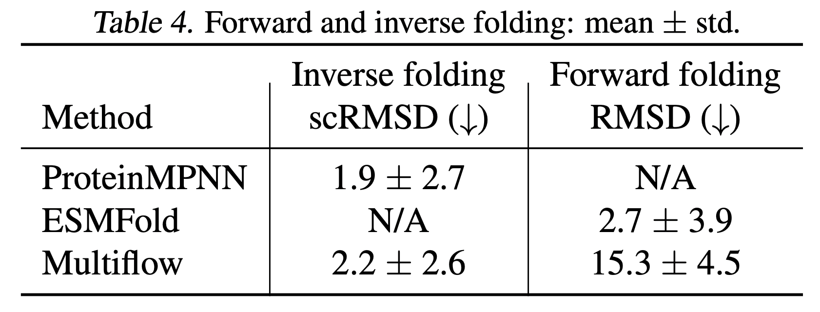
Forward and inverse folding

@article{campbell2024generative,
  title={Generative flows on discrete state-spaces: Enabling multimodal flows with applications to protein co-design},
  author={Campbell, Andrew and Yim, Jason and Barzilay, Regina and Rainforth, Tom and Jaakkola, Tommi},
  journal={arXiv preprint arXiv:2402.04997},
  year={2024}
}