Accurate structure prediction of biomolecular interactions with AlphaFold 3
Technical Details
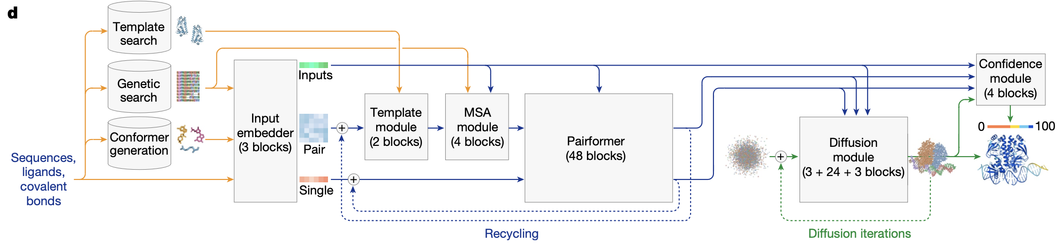
Pairformer
What it is: a streamlined successor to the Evoformer. It iterates attention and triangular updates over the single and pair features but no longer keeps an MSA axis. Why 48 blocks? Empirically, this depth was the sweet spot in AF2 for capturing long‑range geometry; AF3 preserves it but spends the saved MSA FLOPs on more tokens (all atoms, ligands, nucleic acids).
Recycling loop
As in AlphaFold 2 recycling loop is applied during training (with stop gradient) and inference. Typically four recycles are used.
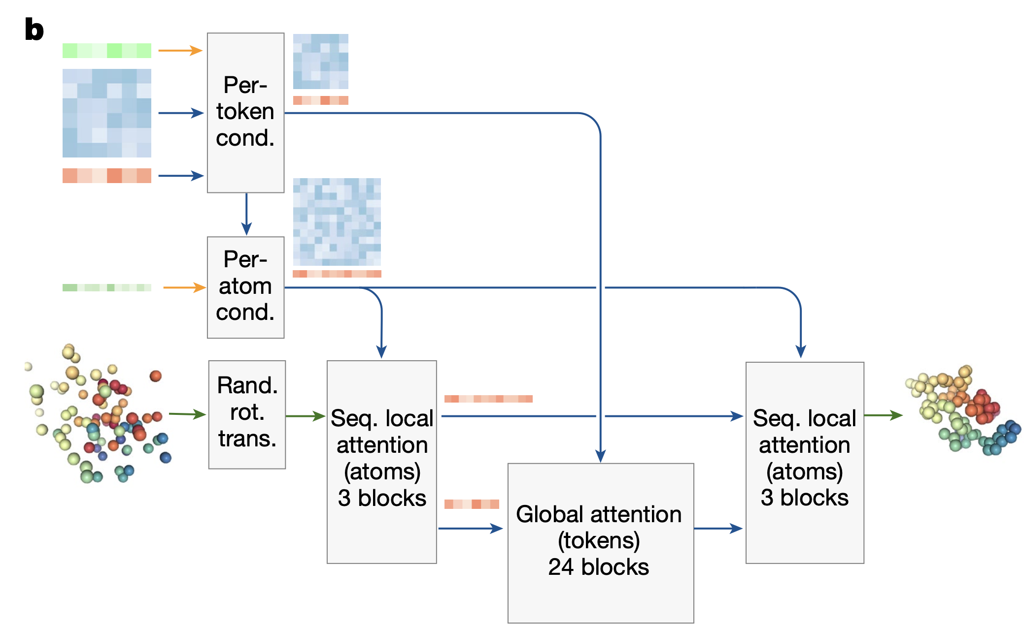
Diffusion model
Diffusion Training
Augmentation
To improve training efficiency the authors train the Diffusion Module with a larger batch size than the trunk. To realise this, they run the trunk once and then create 48 versions of the input structure by randomly rotating and translating according to Algorithm 19 and adding independent noise to each structure.
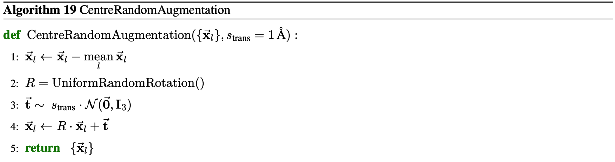
Then the forward diffusion is applied to all augmented samples.
Forward diffusion
P_mean = -1.2,         # mean of log-normal distribution from which noise is drawn for training
P_std = 1.5,           # standard deviation of log-normal distribution from which noise is drawn for training
sigma_min = 0.002,     # min noise level
sigma_max = 80,        # max noise level
sigma_data = 0.5,      # standard deviation of data distribution

def noise_distribution(self, batch_size):
    return (self.P_mean + self.P_std * torch.randn((batch_size,), device = self.device)).exp() * self.sigma_data

sigmas = self.noise_distribution(batch_size).type(dtype)
padded_sigmas = rearrange(sigmas, 'b -> b 1 1')

noise = torch.randn_like(atom_pos_ground_truth)

noised_atom_pos = atom_pos_ground_truth + padded_sigmas * noise  # alphas are 1. in the paper
Schedule:
\[\log \frac{\sigma}{\sigma*{\text{data}}} \sim \mathcal{N}(P*{\text{mean}}, P\_{\text{std}}^2)\]Losses
In this section $\vec{x}_l$ means the denoised structure (diffusion model output).
The authors apply a weighted aligned MSE loss to the denoised structure output from the Diffusion Module. They first perform a rigid alignment of the ground truth $\vec{x}^{\text{GT}}_l$ onto the denoised structure $\vec{x}_l$ as
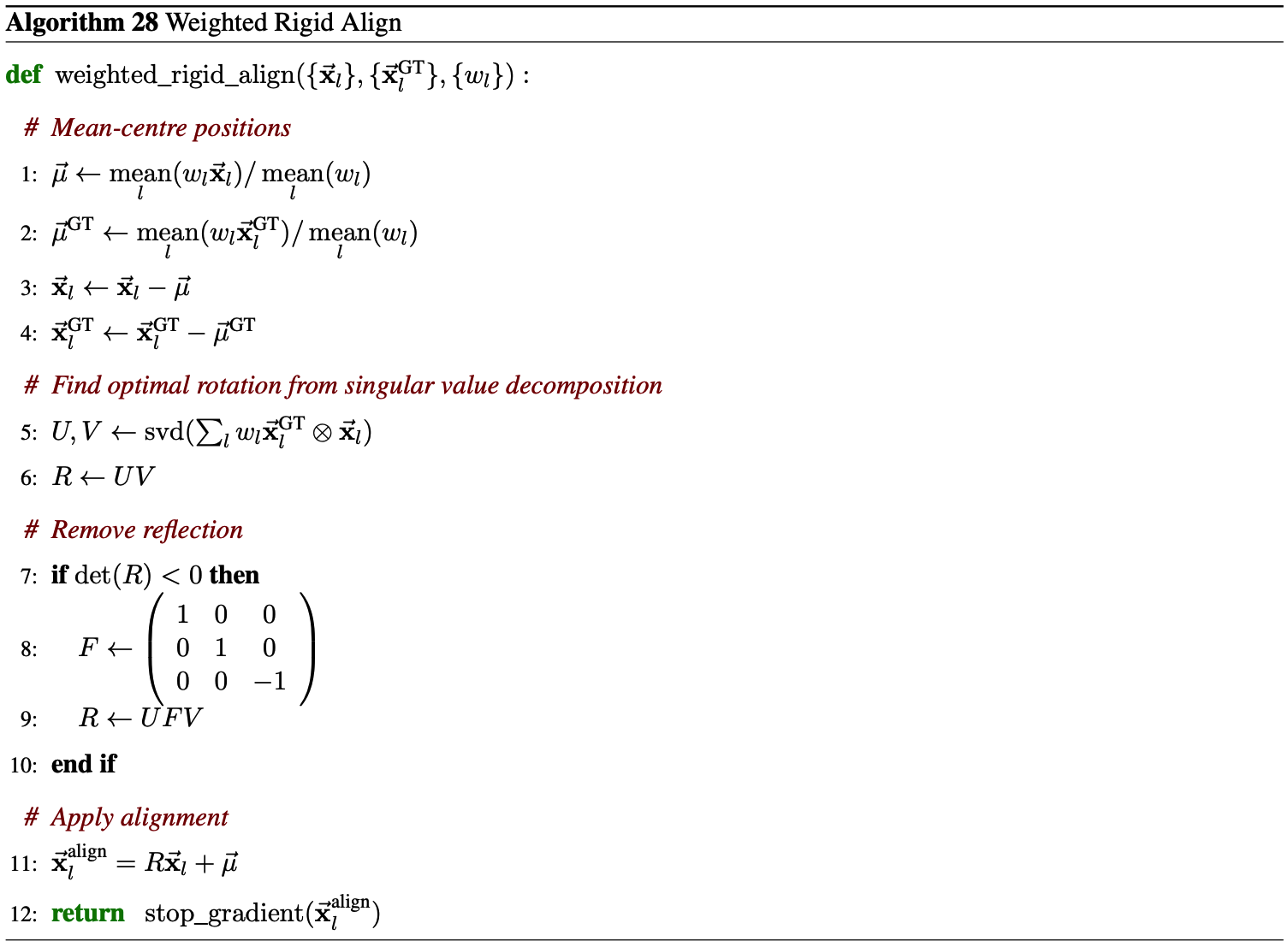
with weights $w_l$ provided in Equation 4. They then compute a weighted MSE
\begin{equation} \mathcal{L}_{\text{MSE}} = \frac{1}{3} \, \text{mean}_l \left( w_l \left| \vec{x}_l - \vec{x}^{\text{GT-aligned}}_l \right|^2 \right) \tag{3} \end{equation}
with upweighting of nucleotide and ligand atoms as
\begin{equation} w_l = 1 + f_l^{\text{is_dna}} \alpha^{\text{dna}} + f_l^{\text{is_rna}} \alpha^{\text{rna}} + f_l^{\text{is_ligand}} \alpha^{\text{ligand}} \tag{4} \end{equation}
and hyperparameters $\alpha^{\text{dna}} = \alpha^{\text{rna}} = 5$, and $\alpha^{\text{ligand}} = 10$.
To ensure that the bonds for bonded ligands (including bonded glycans) have the correct length, the authors introduce an auxiliary loss during fine tuning as
\[\begin{equation} \mathcal{L}_{\text{bond}} = \text{mean}_{(l, m) \in \mathcal{B}} \left( \left\| \vec{x}_l - \vec{x}_m \right\| - \left\| \vec{x}^{\text{GT}}_l - \vec{x}^{\text{GT}}_m \right\| \right)^2 \tag{5} \end{equation}\]where $\mathcal{B}$ is the set of tuples (start atom index, end atom index) defining the bond between the bonded ligand and its parent chain.
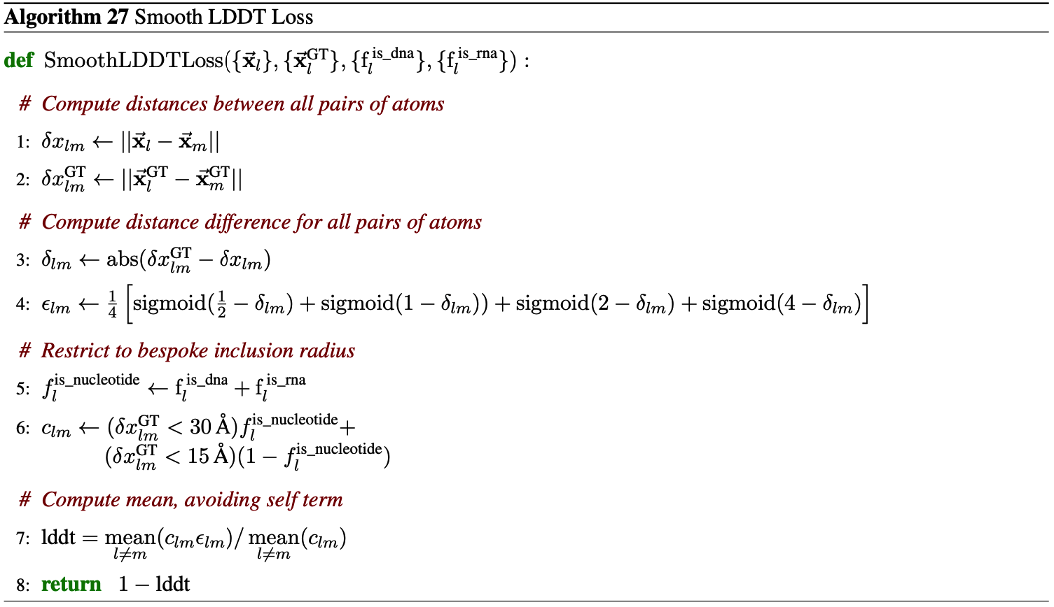
The authors also apply an auxiliary structure-based loss based on smooth LDDT, as described in Algorithm 27. The final loss from the Diffusion Module is then:
\[\begin{equation} \mathcal{L}_{\text{diffusion}} = \frac{\hat{t}^2 + \sigma^2_{\text{data}}}{(\hat{t} + \sigma_{\text{data}})^2} \cdot \left( \mathcal{L}_{\text{MSE}} + \alpha_{\text{bond}} \cdot \mathcal{L}_{\text{bond}} \right) + \mathcal{L}_{\text{smooth\_lddt}} \tag{6} \end{equation}\]Where $\hat{t}$ is the sampled noise level, $\sigma_{\text{data}}$ is a constant determined by the variance of the data (set to 16), and $\alpha_{\text{bond}}$ is 0 for regular training and 1 for both fine tuning stages. Prior to computing the losses, the authors apply an optimal ground truth chain assignment as described in subsection 4.2.
During inference the noise schedule is defined as \begin{equation} \hat{t} = \sigma{\text{data}} \cdot \left( s{\max}^{1/p} + t \cdot (s{\min}^{1/p} - s{\max}^{1/p}) \right)^p \tag{7} \end{equation}
where $s_{\max} = 160$, $s_{\min} = 4 \cdot 10^{-4}$, $p = 7$, and $t$ is distributed uniformly between $[0, 1]$ with a step size of $\frac{1}{200}$.
Architecture